A quick introduction to MetaboCrates • MetaboCrates

Introduction

The MetaboCrates package contains tools for processing and analyzing Biocrates® metabolomics data. It allows users to easily upload data and perform automated preprocessing, including data cleaning, imputation of missing values, and checking the dataset’s comprehensiveness. Additionally, it offers tools for quality control and calculating descriptive statistics, and allows users to quickly save the results.

Getting started

The package can be easily installed and loaded into the environment using the commands:

devtools::install_github("BioGenies/MetaboCrates")

library(MetaboCrates)

Then, the Biocrates® data can be imported with the read_data() function. In this guide an example dataset, included in the package, will be used.

path <- get_example_data("two_sets_example.xlsx")
dat <- read_data(path)

get_info(dat)
#> [1] "Data contains 13 sample types and 2 NA types."

Class of the dat object is both data.frame and raw_data. It has following attributes:

LOD_table - LOD, LLOQ and ULOQ table
NA_info
- counts - types of missing values found in data with their counts
- NA_ratios_type - fractions of missing values of each type per every metabolite
- NA_ratios_group - fractions of missing values with respect to the declared group levels per every metabolite
metabolites - names of metabolites in data
samples - names of sample types with counts
group - a name of grouping column (appears after using add_group() function)
removed - names of removed metabolites
completed - completed data (appears after imputation)
cv - coefficients of variation based on QC sample type for each metabolite (appears after using calculate_CV() function).

Non-null attributes at this stage are presented below.

attr(dat, "LOD_table")[,1:5]
#>                    plate bar code     C0     C2     C3 C3-DC (C4-OH)
#> 1   LOD (calc.) 1052125775-1 [µM]     NA     NA     NA            NA
#> 2   LOD (calc.) 1052125780-1 [µM] 0.7702 0.0545 0.0000        0.0206
#> 3   LOD (calc.) 1052126590-1 [µM]     NA     NA     NA            NA
#> 4   LOD (calc.) 1052126601-1 [µM] 1.4720 0.0269 0.0000        0.0002
#> 5 LOD (from OP) 1052125775-1 [µM]     NA     NA     NA            NA
#> 6 LOD (from OP) 1052125780-1 [µM] 1.6670 0.1333 0.1222        0.0900
#> 7 LOD (from OP) 1052126590-1 [µM]     NA     NA     NA            NA
#> 8 LOD (from OP) 1052126601-1 [µM] 1.6670 0.1333 0.1222        0.0900

attr(dat, "NA_info")[["NA_ratios"]][5:10,]
#> NULL
attr(dat, "NA_info")[["counts"]]
#> # A tibble: 2 × 2
#>   type      n
#>   <chr> <dbl>
#> 1 < LOD 16240
#> 2 NA      316

attr(dat, "metabolites")[1:10]
#>  [1] "C0"            "C2"            "C3"            "C3-DC (C4-OH)"
#>  [5] "C3-OH"         "C3:1"          "C4"            "C4:1"         
#>  [9] "C5"            "C5-DC (C6-OH)"

attr(dat, "samples")[1:5,]
#> # A tibble: 5 × 2
#>   `sample type` count
#>   <chr>         <int>
#> 1 Blank             1
#> 2 QC Level 1        2
#> 3 QC Level 2        6
#> 4 QC Level 3        2
#> 5 Sample          159

Now, information about missing values can be displayed.

attr(dat, "NA_info")[["counts"]]
#> # A tibble: 2 × 2
#>   type      n
#>   <chr> <dbl>
#> 1 < LOD 16240
#> 2 NA      316

plot_mv_types(dat)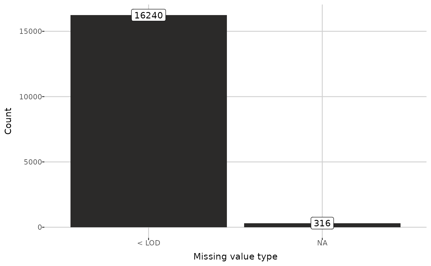

The next step is data preprocessing.

Preprocessing

First, let’s specify a grouping column, which can’t contain any missing values (NA’s). Although this step isn’t necessary, some of the tools require a grouped data.

grouped_dat <- add_group(dat, "submission name")

After grouping,NA_info attribute contains missing values ratios in group levels for each metabolite. Moreover, the grouping column name is added to the group attribute.

attr(grouped_dat, "NA_info")[["NA_ratios"]][5:10,]
#> NULL

attr(grouped_dat, "group")
#> [1] "submission name"

Below, the information about grouped data are displayed.

get_info(grouped_dat)
#> [1] "Data contains 13 sample types and 2 NA types.\nGroupping by: \"submission name\" ( levels)."

plot_groups(grouped_dat)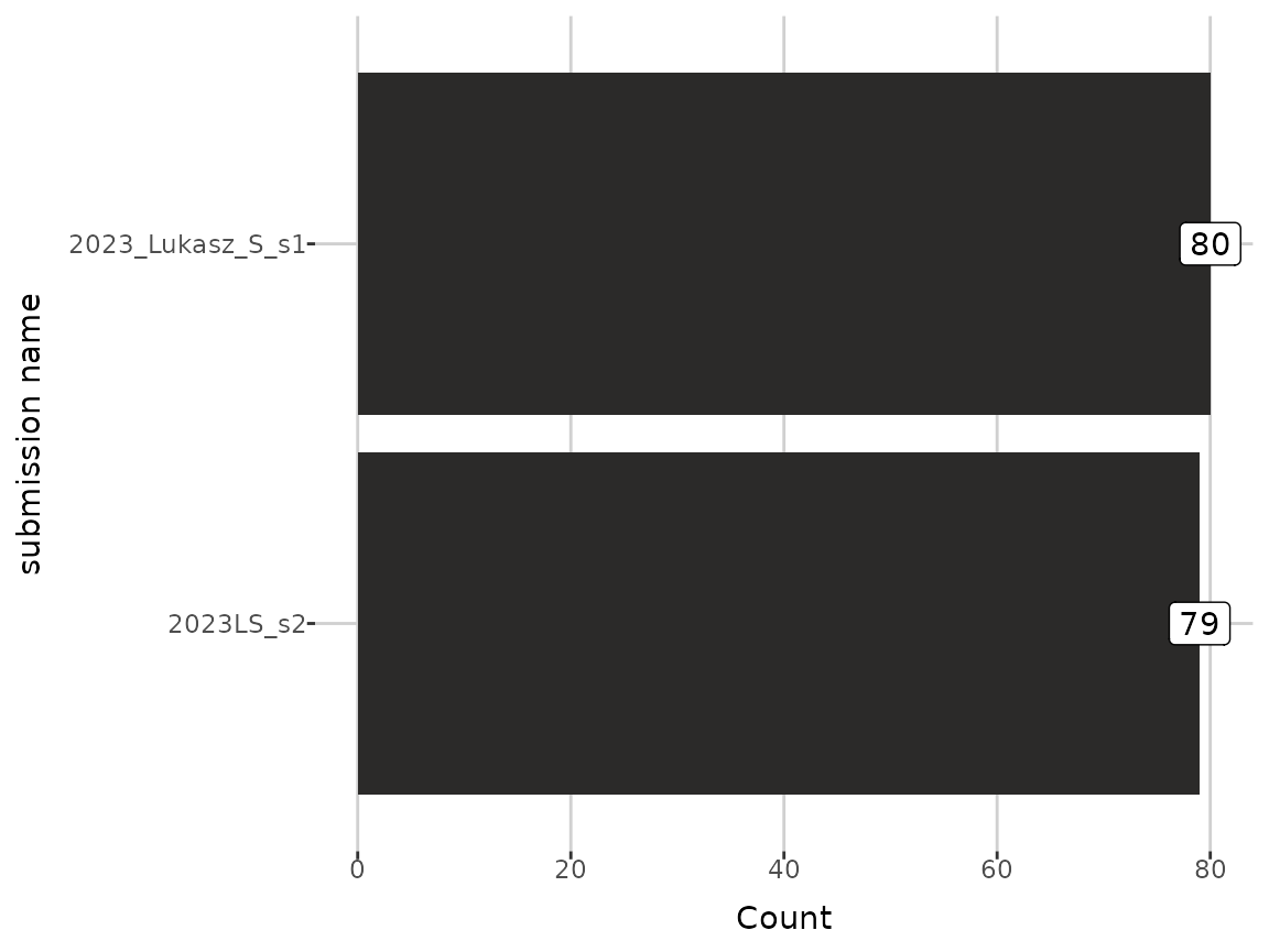

Next, let’s focus on the clearance of data. When ugrouped data passed, function below returns the names of metabolites which have more than the given threshold of missing values. If the grouping column is specified, then it returnes only metabolites for which the threshold is exceeded in each group level. In the examples below the threshold is 20%.

get_LOD_to_remove(dat, 0.2)[1:10]
#> No group to use! It will be ignored.
#>             If you want to use group provide it with add_group function first.
#>  [1] "AbsAcid"  "Ac-Orn"   "Anserine" "BABA"     "C10:1"    "C10:2"   
#>  [7] "C12-DC"   "C12:1"    "C14"      "C14:1-OH"

get_LOD_to_remove(grouped_dat, 0.2)[1:10]
#>  [1] "AbsAcid"  "Ac-Orn"   "Anserine" "C10:1"    "C10:2"    "C12-DC"  
#>  [7] "C12:1"    "C14"      "C14:2"    "C14:2-OH"

Aside from removing metabolites, the data imputation can be also performed, using the complete_data() function. It completes missing values related to limits of quantification or detection. Imputation of each missing value type can be performed with one of five ways:

NULL - skipping imputation
halfmin - half of the minimum observed value
halflimit - half of the detection limit
random - random number not smaller than the limit of detection and not bigger than the minimum observed value
limit - detection limit.

Completed dataset is then stored as the completed attribute.

comp_dat <- complete_data(grouped_dat, LOD_method = "limit")
#> Completing 16240 < LOD values...
#> No < LLOQ values found.
#> No > ULOQ values found.

Getting metabolites to remove can be also based on the coefficient of variation value. In the following example, metabolites with CV value greater than 0.8 are returned.

comp_dat <- calculate_CV(comp_dat)

get_CV_to_remove(comp_dat, 0.8)[1:10]
#>  [1] "C16:2"             "C18:2"             "C3:1"             
#>  [4] "C4:1"              "C5-OH (C3-DC-M)"   "C7-DC"            
#>  [7] "Cer d18:1/18:0-OH" "Cer d18:1/26:1"    "Cer d18:2/18:0"   
#> [10] "Cer d18:2/18:1"

To remove the metabolites from data, the function below can be used. Instead of actually removing them from data, this function adds provided metabolites to the removed attribute. Additionaly, the type of removal can be specified - either LOD, QC or QC_man.

dat_with_metabo_removed <- remove_metabolites(comp_dat, c("C8", "C10"), "LOD")
dat_with_metabo_removed <- remove_metabolites(dat_with_metabo_removed, c("C8", "C12:1"), "QC_man")

attr(dat_with_metabo_removed, "removed")
#> $LOD
#> [1] "C8"  "C10"
#> 
#> $QC
#> NULL
#> 
#> $QC_man
#> [1] "C8"    "C12:1"

Then, the data and LOD ratios without removed metabolites can be displayed. Below, the first 10 rows of both tibbles and chosen columns of the first are visible.

show_data(dat_with_metabo_removed)[1:5, c(1:3, 19:21)]
#>                plate bar code sample bar code sample type    C2     C3
#> 1 1052126590-1 | 1052126601-1        10000001       Blank    NA     NA
#> 2 1052125775-1 | 1052125780-1      1020527268  QC Level 1 1.999 0.7022
#> 3 1052126590-1 | 1052126601-1      1020527268  QC Level 1 2.083 0.7166
#> 4 1052125775-1 | 1052125780-1      1020527272  QC Level 2 3.689  1.461
#> 5 1052125775-1 | 1052125780-1      1020527272  QC Level 2 3.088  1.369
#>   C3-DC (C4-OH)
#> 1            NA
#> 2         < LOD
#> 3        0.0134
#> 4        0.0346
#> 5        0.0344

show_ratios(dat_with_metabo_removed)[7:12,]
#> # A tibble: 6 × 2
#>   metabolite NA_frac
#>   <chr>        <dbl>
#> 1 ADMA         0    
#> 2 AbsAcid      1    
#> 3 Ac-Orn       1    
#> 4 AconAcid     0    
#> 5 Ala          0    
#> 6 Anserine     0.943

There are two options for unremoving metabolites - either the specific ones are can be chosen or all metabolites from the specified type can be restored.

attr(unremove_metabolites(dat_with_metabo_removed, "C8"), "removed")
#> $LOD
#> [1] "C10"
#> 
#> $QC
#> NULL
#> 
#> $QC_man
#> [1] "C12:1"

attr(unremove_all(dat_with_metabo_removed, "QC_man"), "removed")
#> $LOD
#> [1] "C8"  "C10"
#> 
#> $QC
#> NULL
#> 
#> $QC_man
#> NULL

Quality control

The function below creates the PCA plot with respect to the sample type.

create_PCA_plot(comp_dat)
#> Joining with `by = join_by(tmp_id)`
#> Too few points to calculate an ellipse
#> Too few points to calculate an ellipse
#> Warning: Removed 2 rows containing missing values or values outside the scale range
#> (`geom_path()`).

Analysis

First, let’s create the barplots of missing values percents. Below function takes an argument type, which can be set to joined (deafult) to get a plot of missing values in each metabolite or else NA_type or group to add the division into all missing values types and levels in grouping column respectively.

library(ggplot2)

plot_NA_percent(grouped_dat) +
  xlim(attr(grouped_dat, "metabolites")[5:10])
#> NULL

plot_NA_percent(grouped_dat, type = "NA_type") +
  xlim(attr(grouped_dat, "metabolites")[5:10])
#> NULL

plot_NA_percent(grouped_dat, type = "group") +
  xlim(attr(grouped_dat, "metabolites")[5:10])
#> NULL

Next function creates heatmap, which shows if value is missing for each sample and metabolite. Below the cropped plot is presented, with the metabolites from 5th to 10th and first 50 samples.

# plot_heatmap(dat) +
#   xlim(c(0, 50)) +
#   ylim(attr(grouped_dat, "metabolites")[5:10])

Moreover, the heatmap of correlations between all metabolites can be created, using the below function.

create_correlations_heatmap(comp_dat) +
  xlim(attr(comp_dat, "metabolites")[5:10]) +
  ylim(attr(comp_dat, "metabolites")[5:10])
#> NULL

Aside from plots corresponding to the all metabolites, MetaboCrates package provides also tools for visualisations related to the specific metabolite. Next three functions create histogram, boxplot and qqplot, based on the values measured for one metabolite.

Moreover, the package allows for creating the density plot for a specific metabolite, with a dash line representing the limit of detection retrevied from the LOD table.

Next, one can create a beeswarm plot for a specified metabolite, visualizing the distribution of metabolite values across different plate bar codes.

Another function creates a scatter plot of two metabolites values pairs. It also incorporates information about plate bar code and limit of detection values.

create_plot_of_2_metabolites(comp_dat, "C0", "C8")
#> Warning: Removed 1 row containing missing values or values outside the scale range
#> (`geom_interactive_point()`).

Next tool allows for creating a barplot, showing the minimum number of the greatest variances explained by each principal component from a Principal Component Analysis, which cumulative sum is less or equal than given threshold. The plot also includes a line graph representing the cumulative variance explained by the components. Below, the threshold was set to 80%.

pca_variance(comp_dat, 0.8)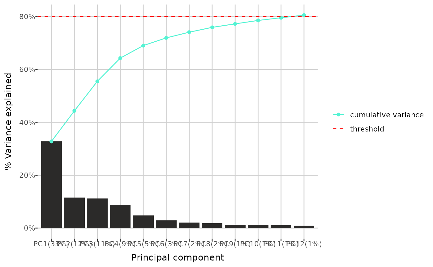

Other Principal Component Analysis tool is the create_pca_plot() function, mentioned in the Quality control section. Its argument type can be set as group, which creates a PCA plot with respect to the specified group levels.

create_PCA_plot(comp_dat, type = "group")
#> Joining with `by = join_by(tmp_id)`
#> Too few points to calculate an ellipse
#> Too few points to calculate an ellipse
#> Warning: Removed 2 rows containing missing values or values outside the scale range
#> (`geom_path()`).