A quick introduction to MetaboCrates • MetaboCrates

Introduction

The MetaboCrates package provides tools for processing and analyzing targeted metabolomics data (e.g., generated using Biocrates® kits). You can easily upload data and perform automated preprocessing, such as data cleaning and missing value imputation, followed by visualizations and descriptive statistics for data exploration. The package also includes tools for quality control, outlier detection and prediction.

Getting started

MetaboCrates can be easily installed and loaded into the environment using the following commands.

devtools::install_github("BioGenies/MetaboCrates")

library(MetaboCrates)

Next, metabolomics data can be imported with the read_data() function. In this guide, an example dataset included in the package will be used.

path <- get_example_data("two_sets_example.xlsx")
dat <- read_data(path)

get_info(dat)
#> [1] "Data contains 13 sample types and 2 NA types."

The class of the dat object is both data.frame and raw_data. It has the following attributes:

LOD_table - table containing the limits of detection (LOD), lower limit of quantification (LLOQ), and upper limit of quantification (ULOQ).
NA_info
- counts - types of missing values found in the data with their counts,
- NA_ratios_type - fractions of missing values of each type for every metabolite,
- NA_ratios_group - fractions of missing values with respect to group levels for every metabolite,
metabolites - names of metabolites in the data,
samples - names of sample types with counts,
group - names of grouping columns (appears after using the add_group() function),
removed - names of metabolites removed based on the:
- LOD - proportion of missing values,
- QC - coefficient of variation (CV),
completed - completed data (appears after imputation),
cv - coefficients of variation based on QC sample type for each metabolite (appears after using the calculate_CV() function).

Non-null attributes at this stage are shown below.

attr(dat, "LOD_table")[,1:5]
#>                    plate bar code     C0     C2     C3 C3-DC (C4-OH)
#> 1   LOD (calc.) 1052125775-1 [µM]     NA     NA     NA            NA
#> 2   LOD (calc.) 1052125780-1 [µM] 0.7702 0.0545 0.0000        0.0206
#> 3   LOD (calc.) 1052126590-1 [µM]     NA     NA     NA            NA
#> 4   LOD (calc.) 1052126601-1 [µM] 1.4720 0.0269 0.0000        0.0002
#> 5 LOD (from OP) 1052125775-1 [µM]     NA     NA     NA            NA
#> 6 LOD (from OP) 1052125780-1 [µM] 1.6670 0.1333 0.1222        0.0900
#> 7 LOD (from OP) 1052126590-1 [µM]     NA     NA     NA            NA
#> 8 LOD (from OP) 1052126601-1 [µM] 1.6670 0.1333 0.1222        0.0900

attr(dat, "NA_info")[["NA_ratios"]][5:10,]
#> NULL
attr(dat, "NA_info")[["counts"]]
#> # A tibble: 2 × 2
#>   type      n
#>   <chr> <dbl>
#> 1 < LOD 16240
#> 2 NA      316

attr(dat, "metabolites")[1:10]
#>  [1] "C0"            "C2"            "C3"            "C3-DC (C4-OH)"
#>  [5] "C3-OH"         "C3:1"          "C4"            "C4:1"         
#>  [9] "C5"            "C5-DC (C6-OH)"

attr(dat, "samples")[1:5,]
#> # A tibble: 5 × 2
#>   `sample type` count
#>   <chr>         <int>
#> 1 Blank             1
#> 2 QC Level 1        2
#> 3 QC Level 2        6
#> 4 QC Level 3        2
#> 5 Sample          159

Now, information about missing values can be displayed.

attr(dat, "NA_info")[["counts"]]
#> # A tibble: 2 × 2
#>   type      n
#>   <chr> <dbl>
#> 1 < LOD 16240
#> 2 NA      316

plot_mv_types(dat)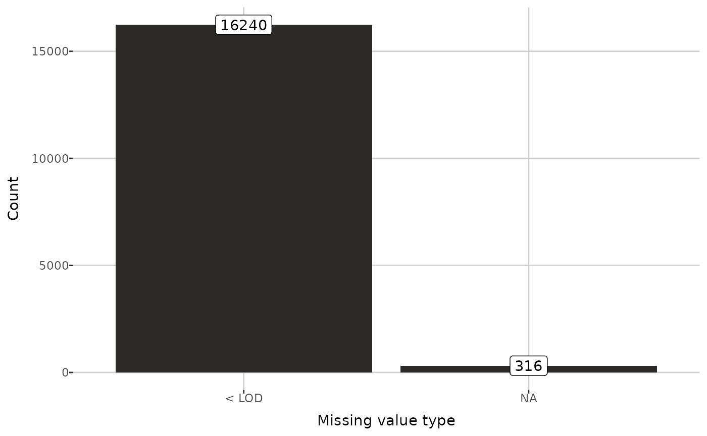

Group selection

Using the add_group() function, you can specify columns (which must not contain any missing values) to group the data by. Although this step is optional, some functions require grouped data.

grouped_dat <- add_group(dat, c("submission name", "species"))

After grouping,the NA_info attribute contains the proportion of missing values in group levels for each metabolite. Moreover, the grouping columns names are added to the group attribute.

attr(grouped_dat, "NA_info")[["NA_ratios_group"]][5:10,]
#> # A tibble: 6 × 3
#>   metabolite grouping_column         NA_frac
#>   <chr>      <chr>                     <dbl>
#> 1 3-IPA      2023LS_s2, human          0    
#> 2 3-IPA      2023_Lukasz_S_s1, human   0    
#> 3 3-Met-His  2023LS_s2, human          0    
#> 4 3-Met-His  2023_Lukasz_S_s1, human   0    
#> 5 5-AVA      2023LS_s2, human          0.114
#> 6 5-AVA      2023_Lukasz_S_s1, human   0.238

attr(grouped_dat, "group")
#> [1] "submission name" "species"

Below, the information about grouped data are displayed.

cat(get_info(grouped_dat))
#> Data contains 13 sample types and 2 NA types.
#> Groupping by: "submission name" (4 levels). Data contains 13 sample types and 2 NA types.
#> Groupping by: "species" (4 levels).

plot_groups(grouped_dat)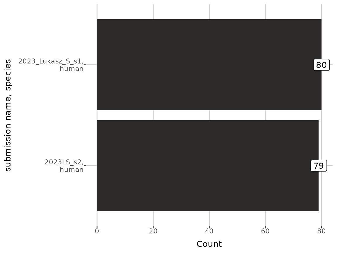

Compounds filtering

To investigate the missing values ratios in each metabolite, the plot_NA_percent() function can be used.

example_metabolites <- c("Cys", "TG 18:3_35:2", "Cortisone", "CDCA", "AbsAcid")

plot_NA_percent(grouped_dat, type = "joint", interactive = FALSE) +
  ylim(example_metabolites)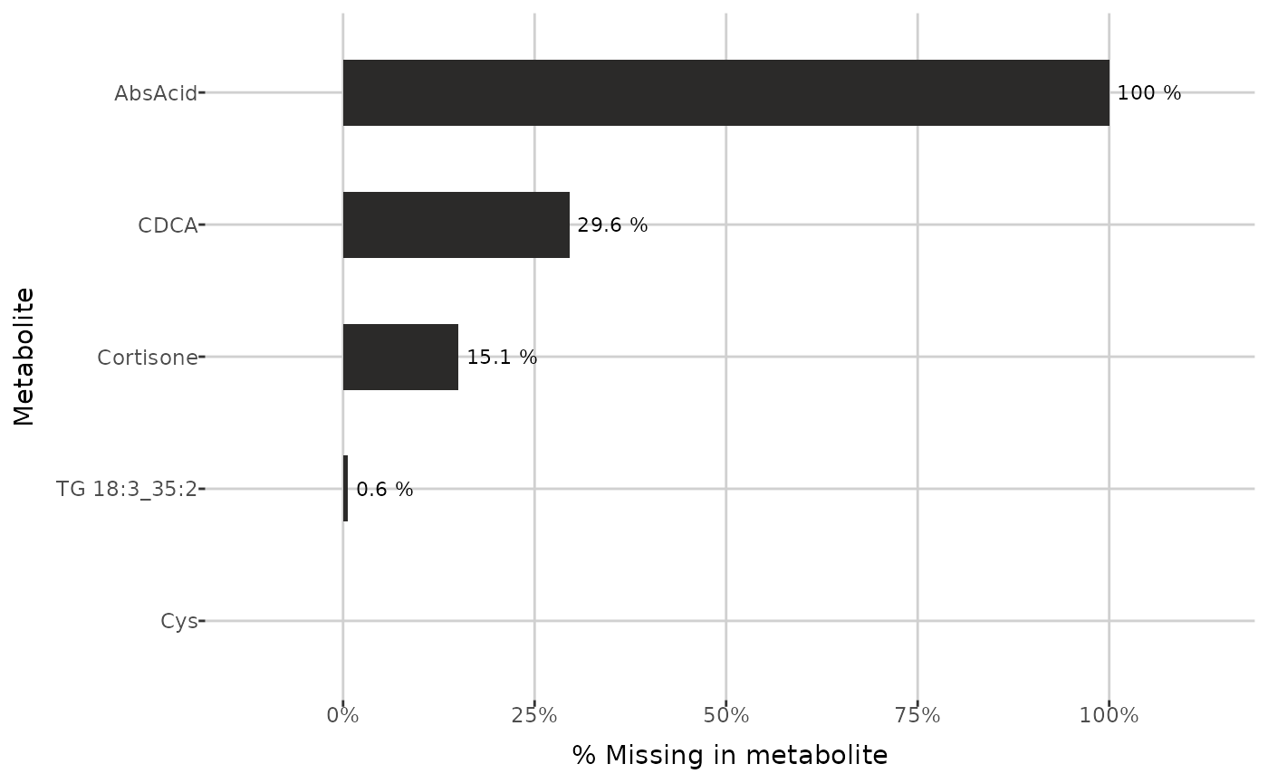


plot_NA_percent(grouped_dat, type = "NA_type", interactive = FALSE) +
  ylim(example_metabolites)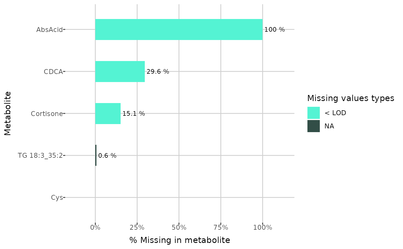


plot_NA_percent(grouped_dat, type = "group", interactive = FALSE) +
  ylim(example_metabolites)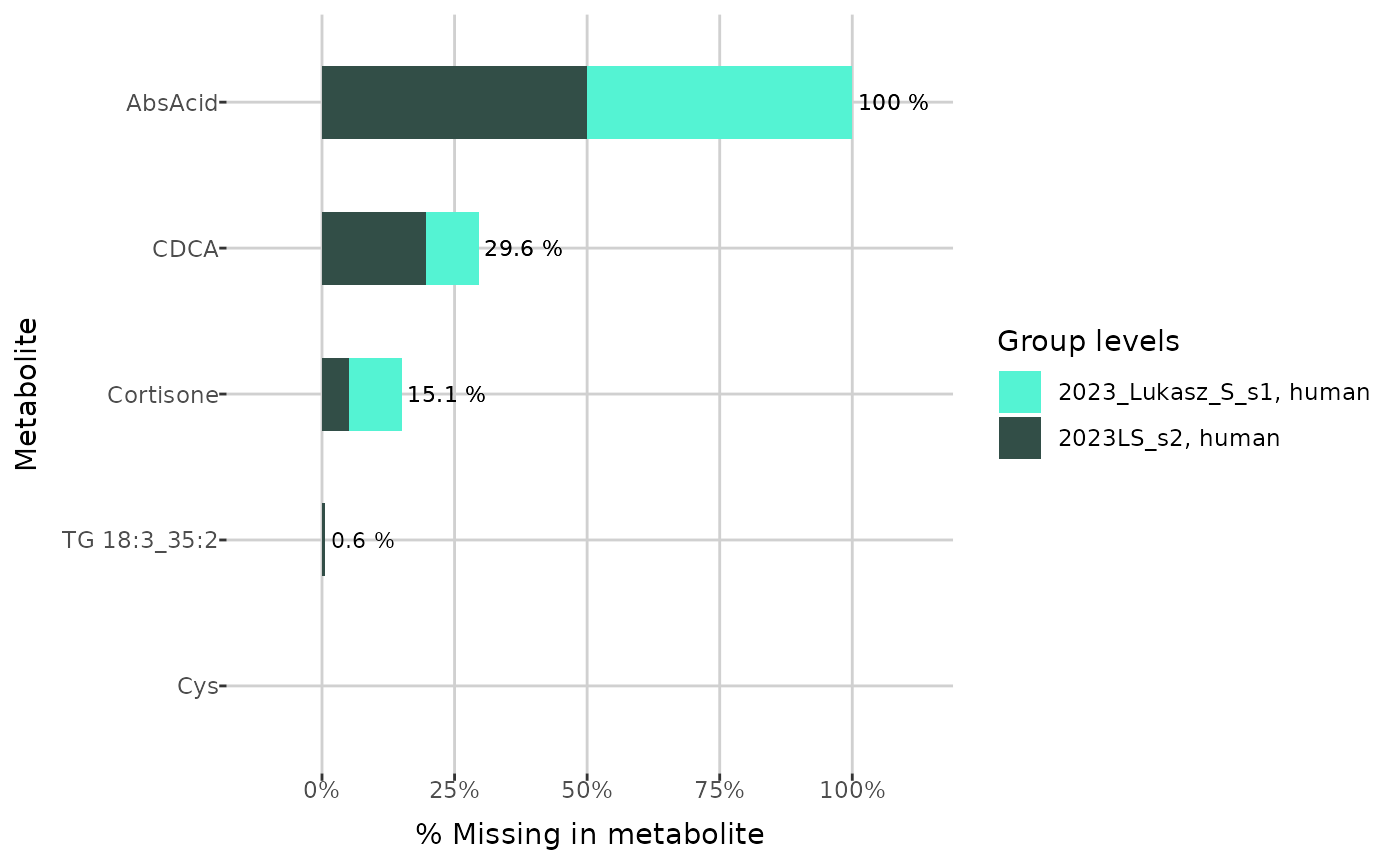

When not grouped data passed, function below returns the names of metabolites which have more than the given threshold of missing values. If the grouping is specified, then it returns only metabolites for which the threshold is exceeded in each group level. In the examples below the threshold is 20%.

get_LOD_to_remove(dat, 0.8)[25:35]
#>  [1] "Carnosine"         "Cer d18:0/18:0"    "Cer d18:0/18:0-OH"
#>  [4] "Cer d18:0/20:0"    "Cer d18:0/26:1"    "Cer d18:1/18:0-OH"
#>  [7] "Cer d18:1/18:1"    "Cer d18:2/18:1"    "DCA"              
#> [10] "DG 16:0_16:0"      "DG 16:0_20:4"

metabolites_to_remove <- get_LOD_to_remove(grouped_dat, 0.8)
metabolites_to_remove[23:33]
#>  [1] "Carnosine"         "Cer d18:0/18:0"    "Cer d18:0/26:1"   
#>  [4] "Cer d18:1/18:0-OH" "Cer d18:1/18:1"    "DCA"              
#>  [7] "DG 16:0_16:0"      "DG 16:1_20:0"      "DG 17:0_17:1"     
#> [10] "DG 18:2_18:4"      "DG 21:0_22:6"

If the grouping with up to 4 levels is specified, then the Venn diagram can be created, which shows the counts of metabolites having ratios of missing values larger than the given threshold for each group level.

create_venn_diagram(grouped_dat, 0.2)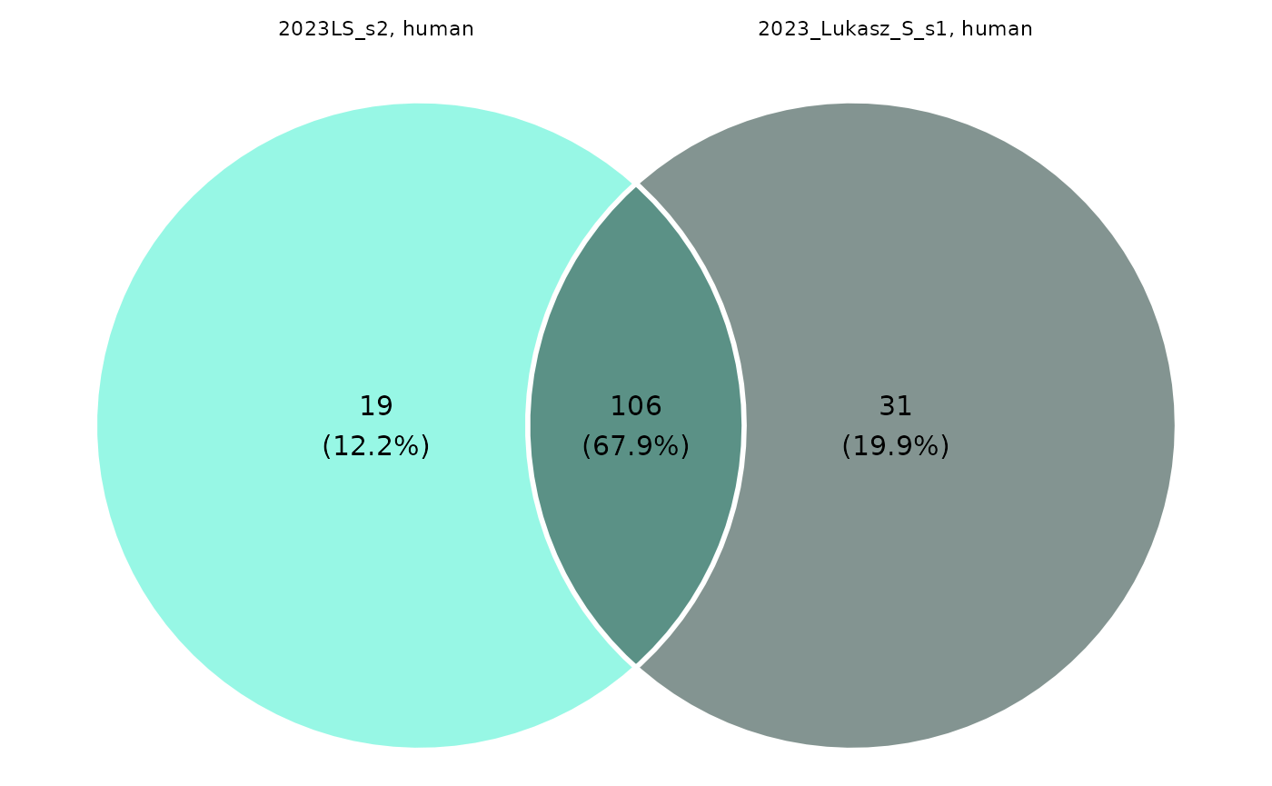

Finally, we can remove the chosen metabolites using the remove_metabolites() function with type specified as LOD. Instead of actually removing them from data, this function adds provided metabolites to the removed attribute.

rm_dat <- remove_metabolites(grouped_dat,
                             metabolites_to_remove = metabolites_to_remove,
                             type = "LOD")

attr(rm_dat, "removed")
#> $LOD
#>  [1] "AbsAcid"            "Ac-Orn"             "Anserine"          
#>  [4] "C10:1"              "C10:2"              "C12-DC"            
#>  [7] "C12:1"              "C14"                "C14:2"             
#> [10] "C16-OH"             "C16:1-OH"           "C16:2-OH"          
#> [13] "C18:1-OH"           "C3-OH"              "C3:1"              
#> [16] "C4:1"               "C5-DC (C6-OH)"      "C5-M-DC"           
#> [19] "C5:1"               "C5:1-DC"            "C6:1"              
#> [22] "C7-DC"              "Carnosine"          "Cer d18:0/18:0"    
#> [25] "Cer d18:0/26:1"     "Cer d18:1/18:0-OH"  "Cer d18:1/18:1"    
#> [28] "DCA"                "DG 16:0_16:0"       "DG 16:1_20:0"      
#> [31] "DG 17:0_17:1"       "DG 18:2_18:4"       "DG 21:0_22:6"      
#> [34] "DG 22:1_22:2"       "DG O-16:0_20:4"     "DiCA(12:0)"        
#> [37] "Dopamine"           "FA 12:0"            "FA 14:0"           
#> [40] "FA 16:0"            "FA 18:0"            "Hex2Cer d18:1/26:0"
#> [43] "Hex3Cer d18:1/26:1" "Indole"             "OH-GlutAcid"       
#> [46] "PAG"                "PC 26:0"            "PC 40:1"           
#> [49] "PC O-42:0"          "PEA"                "SM 40:4"           
#> [52] "Suc"                "TG 18:2_31:0"       "TG 20:1_24:3"      
#> [55] "TG 20:1_31:0"       "TG 20:2_36:5"       "c4-OH-Pro"         
#> 
#> $QC
#> NULL

Then, the data and missing values ratios without removed metabolites can be displayed. Below, the first 5 rows of both tibbles and chosen columns of the first are visible.

show_data(rm_dat)[1:5, c(1:3, 19:21)]
#>                plate bar code sample bar code sample type    C2     C3
#> 1 1052126590-1 | 1052126601-1        10000001       Blank    NA     NA
#> 2 1052125775-1 | 1052125780-1      1020527268  QC Level 1 1.999 0.7022
#> 3 1052126590-1 | 1052126601-1      1020527268  QC Level 1 2.083 0.7166
#> 4 1052125775-1 | 1052125780-1      1020527272  QC Level 2 3.689  1.461
#> 5 1052125775-1 | 1052125780-1      1020527272  QC Level 2 3.088  1.369
#>   C3-DC (C4-OH)
#> 1            NA
#> 2         < LOD
#> 3        0.0134
#> 4        0.0346
#> 5        0.0344

show_ratios(rm_dat)[1:5,]
#> # A tibble: 5 × 2
#>   metabolite NA_frac
#>   <chr>        <dbl>
#> 1 1-Met-His    0    
#> 2 3-IAA        0    
#> 3 3-IPA        0    
#> 4 3-Met-His    0    
#> 5 5-AVA        0.176

There are two options for restoring metabolites - either specific ones can be selected or all metabolites from the specified type can be restored.

attr(unremove_metabolites(rm_dat, "AbsAcid"), "removed")
#> $LOD
#>  [1] "Ac-Orn"             "Anserine"           "C10:1"             
#>  [4] "C10:2"              "C12-DC"             "C12:1"             
#>  [7] "C14"                "C14:2"              "C16-OH"            
#> [10] "C16:1-OH"           "C16:2-OH"           "C18:1-OH"          
#> [13] "C3-OH"              "C3:1"               "C4:1"              
#> [16] "C5-DC (C6-OH)"      "C5-M-DC"            "C5:1"              
#> [19] "C5:1-DC"            "C6:1"               "C7-DC"             
#> [22] "Carnosine"          "Cer d18:0/18:0"     "Cer d18:0/26:1"    
#> [25] "Cer d18:1/18:0-OH"  "Cer d18:1/18:1"     "DCA"               
#> [28] "DG 16:0_16:0"       "DG 16:1_20:0"       "DG 17:0_17:1"      
#> [31] "DG 18:2_18:4"       "DG 21:0_22:6"       "DG 22:1_22:2"      
#> [34] "DG O-16:0_20:4"     "DiCA(12:0)"         "Dopamine"          
#> [37] "FA 12:0"            "FA 14:0"            "FA 16:0"           
#> [40] "FA 18:0"            "Hex2Cer d18:1/26:0" "Hex3Cer d18:1/26:1"
#> [43] "Indole"             "OH-GlutAcid"        "PAG"               
#> [46] "PC 26:0"            "PC 40:1"            "PC O-42:0"         
#> [49] "PEA"                "SM 40:4"            "Suc"               
#> [52] "TG 18:2_31:0"       "TG 20:1_24:3"       "TG 20:1_31:0"      
#> [55] "TG 20:2_36:5"       "c4-OH-Pro"         
#> 
#> $QC
#> NULL

attr(unremove_all(rm_dat, "LOD"), "removed")
#> $LOD
#> NULL
#> 
#> $QC
#> NULL

Gaps completing

Aside from removing metabolites, missing values can be also imputed using the complete_data() function. It completes missing values related to the limits of quantification and detection. Imputation of values below the limit of detection (< LOD) can be performed in one of seven ways:

NULL - skipping imputation,
halfmin - half of the minimum observed value,
halflimit - half of the detection limit,
random - random number not smaller than the limit of detection and not bigger than the minimum observed value,
limit - the detection limit,
limit-0.2min - the detection limit minus 0.2 times the minimum observed value,
logspline - random number from a logspline density fitted to the observed values.

Values below the quantification limit (< LLOQ) can be imputed using either NULL or limit methods. Similarly, values above the upper limit of quantification (> ULOQ) can be imputed using the NULL and limit methods or

third quartile - third quartile of the observed values,
scaled random - random number higher than the upper limit of quantification but lower than its double.

Completed dataset is then stored as the completed attribute.

comp_dat <- complete_data(rm_dat,
                          LOD_method = "halfmin",
                          LLOQ_method = "limit",
                          ULOQ_method = "third quartile")

To investigate missing values, you can use the plot_heatmap() function, which creates a heatmap indicating whether a value is missing for each sample and metabolite, depending on the plate bar code. You can specify a plate bar code to generate a single plot; otherwise, if there are multiple plate bar codes in the dataset, a faceted plot will be created. If show_colors = TRUE, each missing value type is shown in a different color. Below, cropped plots are presented, showing the first five metabolites.

plot_heatmap(comp_dat, plate_bar_code = "1052125775-1 | 1052125780-1") +
   ylim(attr(comp_dat, "metabolites")[5:1])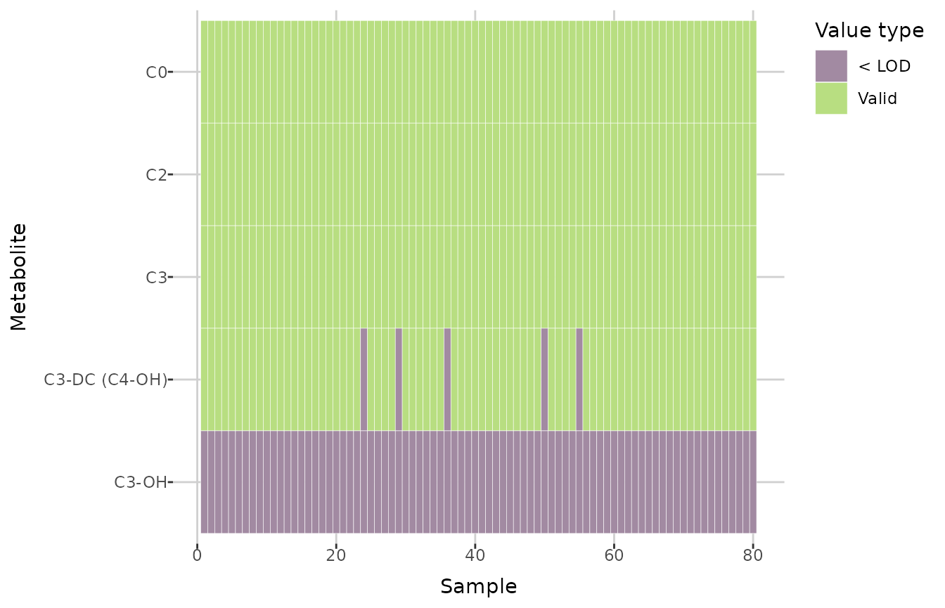


plot_heatmap(comp_dat) +
   ylim(attr(comp_dat, "metabolites")[5:1])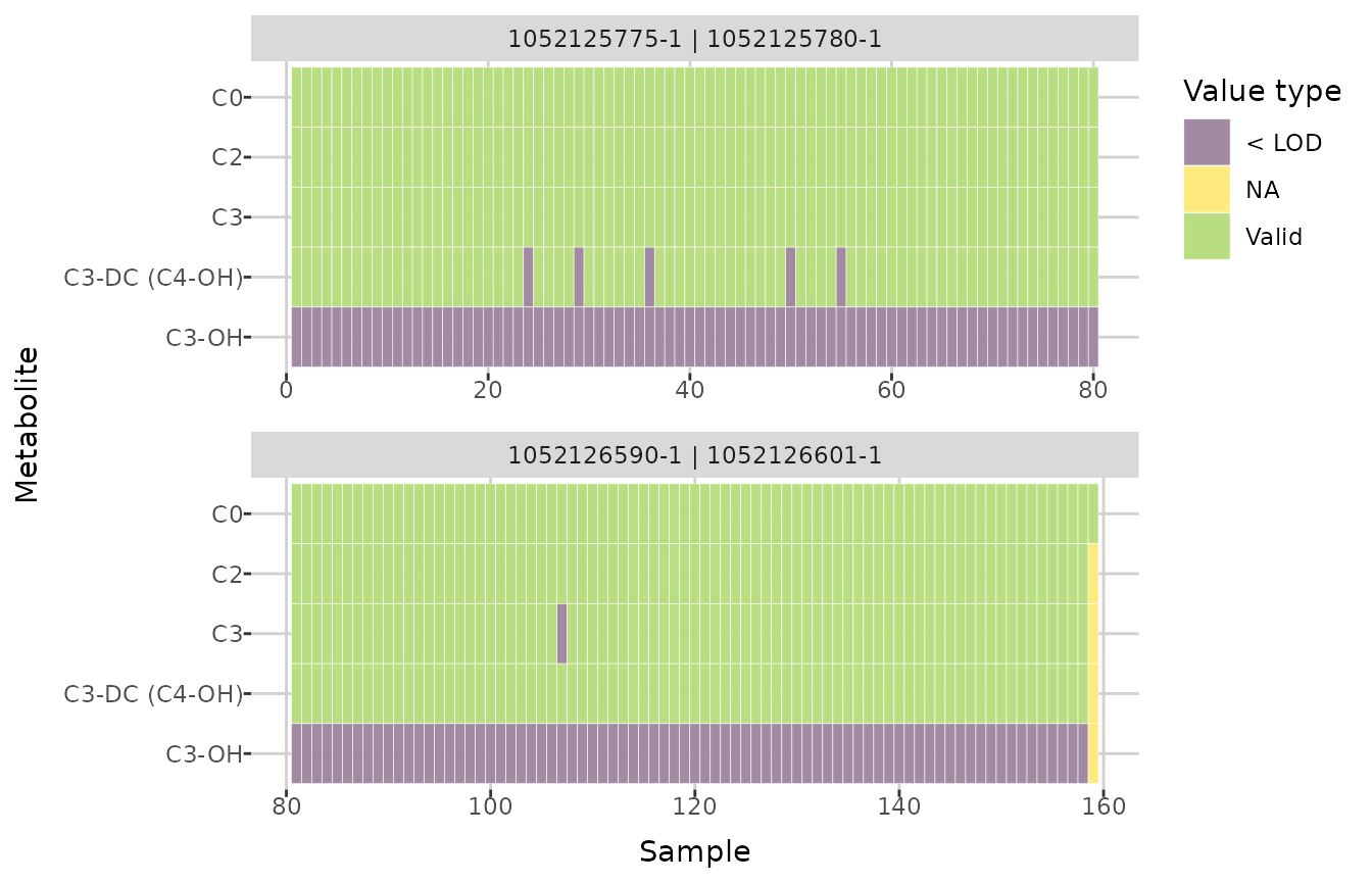

Next, you can compare the distributions of an individual metabolite before and after imputation. The create_distribution_plot() function can generate a histogram, density plot, and beeswarm plot (either regular or interactive with tooltips). Additionally, for histogram, you can choose to display either all values after imputation or only those that were previously missing and then imputed.

create_distribution_plot(comp_dat, metabolite = "C9", bins = 40)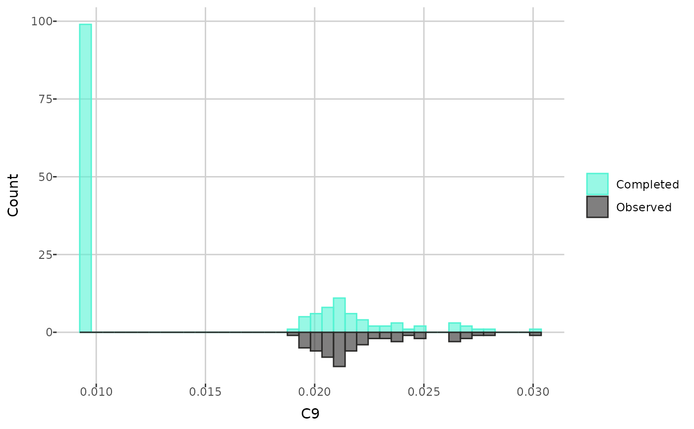


create_distribution_plot(comp_dat, metabolite = "C9", bins = 40,
                         histogram_type = "imputed")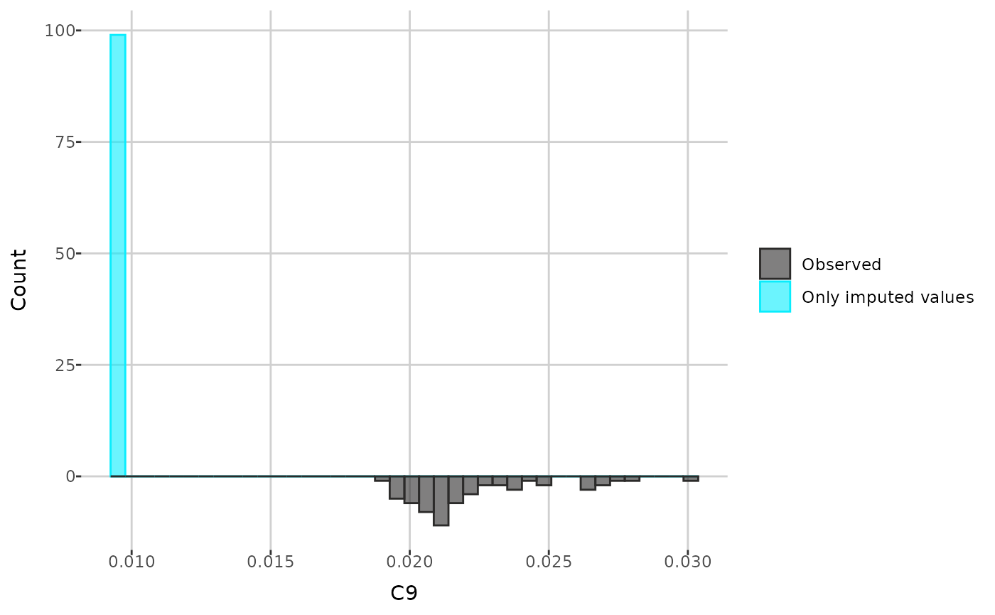


create_distribution_plot(comp_dat, metabolite = "C9", type = "density")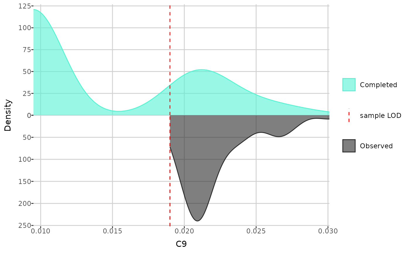


create_distribution_plot(comp_dat, metabolite = "C9",
                         type = "beeswarm")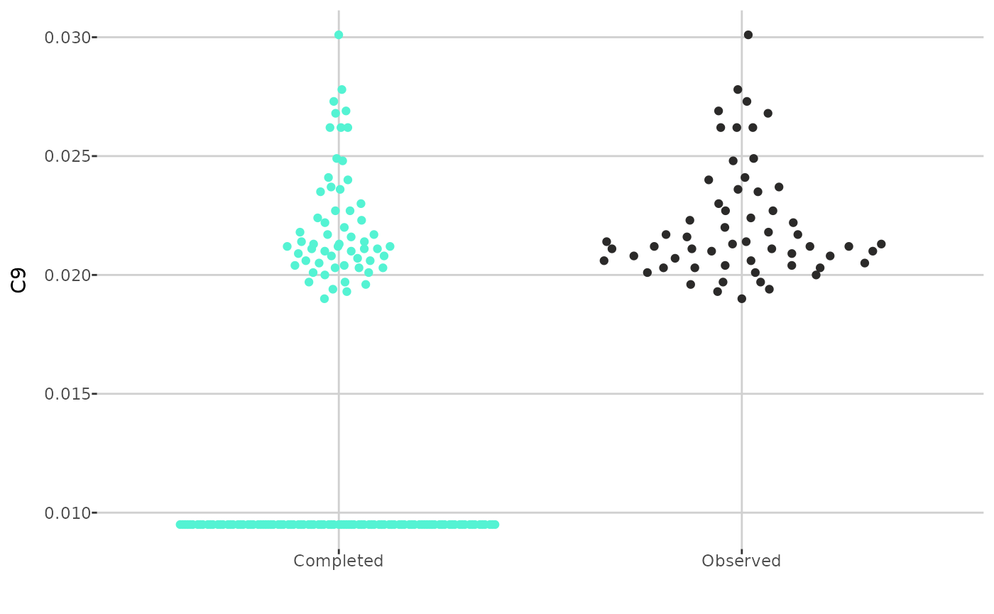

MetaboCrates also offers two types of Q-Q plots: a theoretical Q-Q plot (using the create_qqplot() function), which compares the quantiles of a metabolite with the quantiles of the normal distribution, and an empirical Q-Q plot (with create_empirical_qqplot()), which compares the quantiles of metabolite values before and after imputation.

create_qqplot(comp_dat, metabolite = "C9")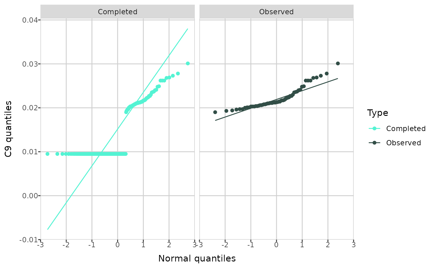


create_empirical_qqplot(comp_dat, metabolite = "C9")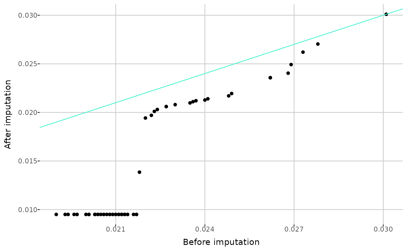

After imputation, you can perform quality control and outlier detection.

Quality control

To perform quality control, you must calculate the coefficients of variation (CV) for each quality control type using the completed data.

qc_dat <- calculate_CV(comp_dat)

The coefficients of variation can now be accessed in the cv attribute.

attr(qc_dat, "cv")[1:5,]
#> # A tibble: 5 × 3
#>   `sample type` metabolite      CV
#>   <chr>         <chr>        <dbl>
#> 1 QC Level 1    1-Met-His  0.0392 
#> 2 QC Level 1    3-IAA      0.00646
#> 3 QC Level 1    3-IPA      0.0252 
#> 4 QC Level 1    3-Met-His  0.0322 
#> 5 QC Level 1    5-AVA      0.0722

You can obtain the metabolites with CV values greater than a specified threshold using the following function.

get_CV_to_remove(qc_dat, 0.8)[1:5]
#> [1] "C14:1"          "C3-DC (C4-OH)"  "Cer d18:1/26:0" "Cer d18:2/18:0"
#> [5] "DG 14:1_18:1"

To remove metabolites from the data, use the remove_metabolites() function.

qc_dat <- remove_metabolites(qc_dat, c("C14:1", "C3-DC (C4-OH)"), "QC")

attr(qc_dat, "removed")
#> $LOD
#>  [1] "AbsAcid"            "Ac-Orn"             "Anserine"          
#>  [4] "C10:1"              "C10:2"              "C12-DC"            
#>  [7] "C12:1"              "C14"                "C14:2"             
#> [10] "C16-OH"             "C16:1-OH"           "C16:2-OH"          
#> [13] "C18:1-OH"           "C3-OH"              "C3:1"              
#> [16] "C4:1"               "C5-DC (C6-OH)"      "C5-M-DC"           
#> [19] "C5:1"               "C5:1-DC"            "C6:1"              
#> [22] "C7-DC"              "Carnosine"          "Cer d18:0/18:0"    
#> [25] "Cer d18:0/26:1"     "Cer d18:1/18:0-OH"  "Cer d18:1/18:1"    
#> [28] "DCA"                "DG 16:0_16:0"       "DG 16:1_20:0"      
#> [31] "DG 17:0_17:1"       "DG 18:2_18:4"       "DG 21:0_22:6"      
#> [34] "DG 22:1_22:2"       "DG O-16:0_20:4"     "DiCA(12:0)"        
#> [37] "Dopamine"           "FA 12:0"            "FA 14:0"           
#> [40] "FA 16:0"            "FA 18:0"            "Hex2Cer d18:1/26:0"
#> [43] "Hex3Cer d18:1/26:1" "Indole"             "OH-GlutAcid"       
#> [46] "PAG"                "PC 26:0"            "PC 40:1"           
#> [49] "PC O-42:0"          "PEA"                "SM 40:4"           
#> [52] "Suc"                "TG 18:2_31:0"       "TG 20:1_24:3"      
#> [55] "TG 20:1_31:0"       "TG 20:2_36:5"       "c4-OH-Pro"         
#> 
#> $QC
#> [1] "C14:1"         "C3-DC (C4-OH)"

Outlier detection

To detect outliers and patterns corresponding to variation in the data, you can use principal component analysis (PCA). MetaboCrates offers several PCA plots. The function below creates PCA scatterplots, which visualize the clustering of observations with respect to the sample type or group level.

create_PCA_plot(qc_dat,
                types_to_display = c("Sample", "QC Level 1", "QC Level 2"))


create_PCA_plot(qc_dat, group_by = "group")

Using the same function, you can also generate biplots (based on data with all sample types if group_by = "sample_type", or only type Sample when group_by = "group"), displaying loadings above a given threshold. This plot type illustrates how each metabolite contributes to the first two principal components and highlights metabolites that capture similar information.

create_PCA_plot(qc_dat, type = "biplot", threshold = 0.05, interactive = FALSE)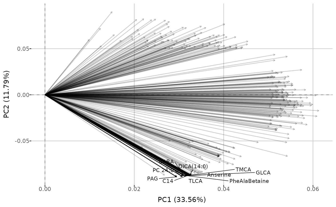


create_PCA_plot(qc_dat, type = "biplot", group_by = "group", threshold = 0.05,
                interactive = FALSE)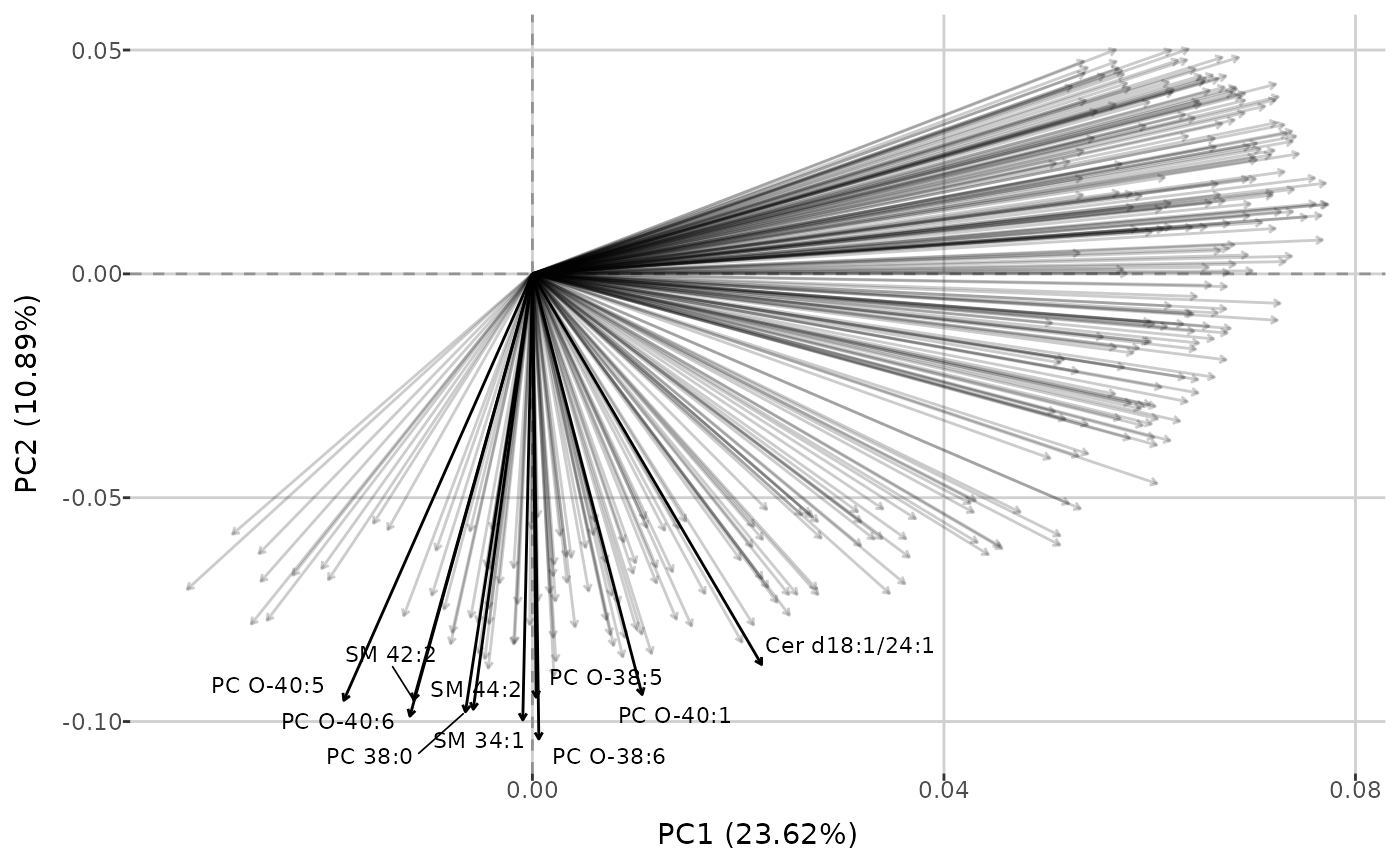

Finally, you can investigate the percentage of total variance in the data explained by each principal component. Additionally, cumulative variance - the sum of the percentage variance contributions from the first principal component up to a given component - can be displayed. Threshold determines which principal components are shown: all components for which the cumulative variance remains below the threshold are included, along with one additional component that brings the cumulative variance just above the threshold (if applicable). You can also specify the maximum number of principal components to display on the plot.

pca_variance(qc_dat, threshold = 0.7)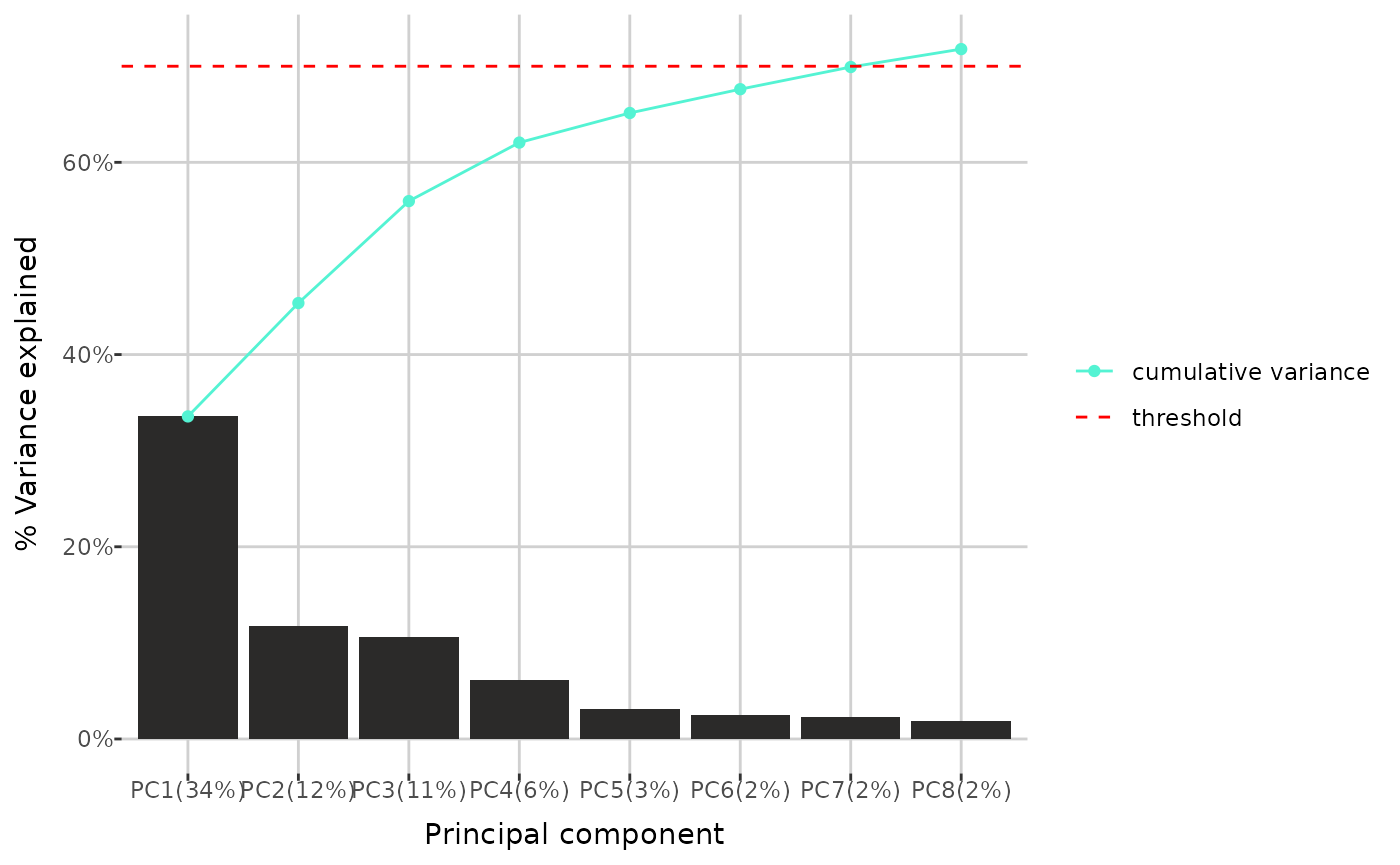


pca_variance(qc_dat, threshold = 0.7, group_by = "group", max_num = 6,
             cumulative = FALSE)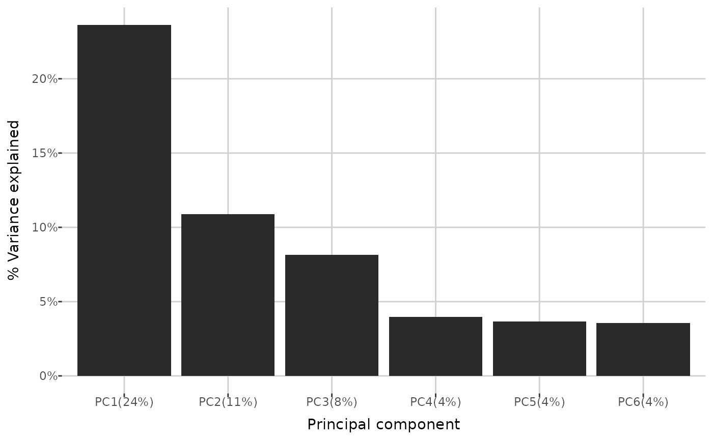

Modeling

Two types of penalized logistic regression models are available: SLOPE (Larsson, Bogdan et al., “Efficient Solvers for SLOPE in R, Python, Julia, and C++.”) and Lasso (Friedman, Hastie, Tibshirani, “Regularization Paths for Generalized Linear Models via Coordinate Descent.”).

You can fit the chosen model, with parameters estimated through cross-validation, using the build_model() function. The response variable must be one of the grouping variables. If the response has more than two levels, the target level must be specified.

model <- build_model(qc_dat, response = "submission name", model = "SLOPE",
                     nfolds = 5, train_prop = 0.6)

get_model_summary() returns a list containing: train dataset, test dataset with predicted values, model coefficients, AUC value and ROC plot.

model_summary <- get_model_summary(model)

model_summary[["train"]][1:5, 1:5]
#>   sample identification 2023LS_s2     C0    C2     C3
#> 2    G0005v6_7512691183         0 10.310 5.089 0.3858
#> 3    G0001v4_7512778233         0  3.943 4.164 0.2052
#> 4    G0007v3_7512803774         0  7.901 8.129 0.3669
#> 5    G0005v3_7512799609         0  7.885 5.012 0.3433
#> 6     RC2224_7508763832         0  4.927 4.005 0.2521

model_summary[["test"]][1:5, 1:6]
#>   probability_2023LS_s2 sample identification 2023LS_s2     C0    C2     C3
#> 1          0.0151803170    G0019v4_7512784194         0 10.670 5.457 0.4434
#> 2          0.0003433938    G0003v6_7512511202         0  7.348 8.286 0.3608
#> 3          0.0010533809    G0004v6_7510389556         0  4.981 3.715 0.2824
#> 4          0.0051978951    G0001v3_7512786908         0  4.224 3.721 0.2186
#> 5          0.0090377723    G0020v6_5010236250         0  5.806 2.972 0.2787

model_summary[["coefficients"]][1:5,]
#>          term      estimate
#> 1 (Intercept)  1.048551e+00
#> 2          C0  1.414565e-01
#> 3    C14:1-OH  1.315262e+02
#> 4    C14:2-OH -5.748579e+01
#> 5         Gln  2.211286e-04

model_summary[["auc"]]
#> [1] 1

model_summary[["roc_plot"]]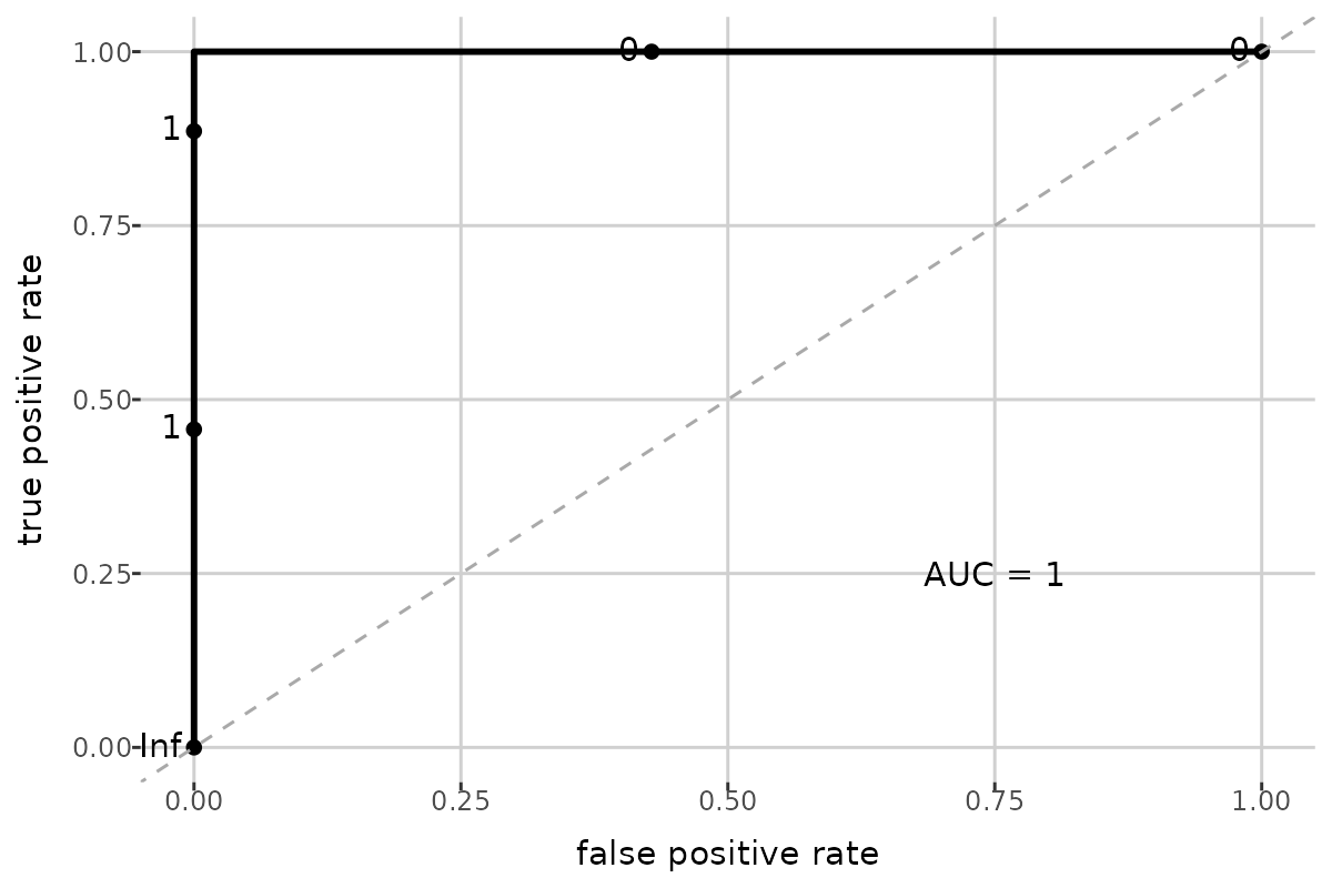

You can also generate predictions for a new dataset by passing a cleaned metabolomics or compounds matrix to the predict_probability() function. If no dataset is provided, predictions for the test dataset are returned.

predict_probability(model, new_dat = NULL)[1:5, 1:6]
#>   probability_2023LS_s2 sample identification 2023LS_s2     C0    C2     C3
#> 1          0.0151803170    G0019v4_7512784194         0 10.670 5.457 0.4434
#> 2          0.0003433938    G0003v6_7512511202         0  7.348 8.286 0.3608
#> 3          0.0010533809    G0004v6_7510389556         0  4.981 3.715 0.2824
#> 4          0.0051978951    G0001v3_7512786908         0  4.224 3.721 0.2186
#> 5          0.0090377723    G0020v6_5010236250         0  5.806 2.972 0.2787